Dickinson Lab
The California Institute of Technology
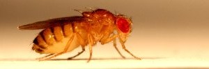
The Dickinson Lab studies the neural and biomechanical basis of behavior in the fruit fly, Drosophila. We strive to build an integrated model of behavior that incorporates an understanding of morphology, neurobiology, muscle physiology, physics, and ecology. Although our research focuses primarily on flight control, we are interested in how animals transform sensory information into a code that controls motor output and behavior.